 Intro to Dimensionality Reduction
Week 7 | Lesson 2.1
LEARNING OBJECTIVES
After this lesson, you will be able to:
- Understand the logical workflow behind dimensionality reduction
- Understand the basic mathematical structure behind dimensionality reduction
- Calculate eigenvectors and eigenvalues for use in Principal Component Analysis
STUDENT PRE-WORK
Before this lesson, you should already be able to:
- Have a working understand of scikit learn and numpy
- Be able to create functions from scratch in python
- Have a basic understanding of linear algebra concepts such as matrices, eigenvalues, and eigenvectors
INSTRUCTOR PREP
Before this lesson, instructors will need to:
- Read in / Review any dataset(s) & starter/solution code
- Generate a brief slide deck
- Prepare any specific materials
- Provide students with additional resources
STARTER CODE
LESSON GUIDE
| TIMING | TYPE | TOPIC |
|---|---|---|
| 5 min | Opening | Opening |
| 10 min | Introduction | Introduction to Dimensionality Reduction |
| 15 min | Demo | Applications of Dimensionality Reduction: A Long-Form Approach |
| 25 min | Guided Practice | Conducting Dimensionality Analysis |
| 25 min | Independent Practice | Dimensionality Reduction on the Iris Dataset |
| 5 min | Conclusion | Conclusion |
Opening (5 mins)
- Review prior labs/homework, upcoming projects, or exit tickets, when applicable
- Review lesson objectives
- Discuss real world relevance of these topics
- Relate topics to the Data Science Workflow - i.e. are these concepts typically used to acquire, parse, clean, mine, refine, model, present, or deploy?
Check: Ask students to define, explain, or recall any relevant prework concepts.
Introduction: What is Dimensionality Reduction? (10 mins)
So you're probably wondering, what is dimensionality reduction? If it sounds like a sci-fi term for transporting into a different "dimension," to a degree you're absolutely correct. You're just transporting your data into a different dimension, not yourself.
Dimensionality reduction reduces the number of random variables that you are considering for analysis until you are left with the most important variables; we want to show data in a simpler and more concise manner.
Dimensionality reduction is not an end goal in itself, but a tool to form a dataset with better features for a classification or regression model.
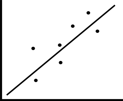
Imagine we have a linear graph, with one variable on the x axis and another on the y axis. If we were to introduce both of these dimensions into a classification or regression model, they would introduce a great deal of noise. So what do we do? We reduce the dimensions until the 45 degree line is completely horizontal - both of our measurements are now on the same plane - they are one-dimensional.

While dimensionality reduction can be a large piece of random forests using a feature selection approach, which you've already explored in previous lessons, we're going to focus on a form of dimensionality reduction known as principal component analysis or PCA that uses feature extraction. Whereas feature selection attempts to discover relevant subsets of the original data, feature extraction dimensionality analysis combines the extraction of key features of a potentially correlated dataset with the dimension reduction described above, resulting in the new, linear non-correlated set.
Check: Check with students to ensure that they understand these concepts at a high level. Have individual students or groups of students define and explain these concepts to the rest of the class
Demo: Applications of Dimensionality Reduction: A long-form approach (20 mins)
While python has many built in applications of dimensionality reduction, such as the PCA approach that we will explore in our next lesson, today we're going to examine the the manual approach to understand the inner workings of the DR.
Before we jump into the actual analysis, we're going to look at the mathematical underworking of dimensionality reduction, leading into the use of the principal component analysis method in the next lesson.
When conducting dimensionality reduction, the first step is to break your dataset into two parts - one set, which we'll call "x" that will be all of the attribute data, and on set called "y" that will be the classes of the dataset.
x = data.ix[selection].values
y = data.ix[selection].values
Here, we are simply selecting the values we want for our variables. Where you see "selection," select the columns that you would like for each value. For instance, if the attributes are in columns 1-8, we write x = data.ix[:,0:7].values.
Next, we'll standardize the data just in case different attributes with been measures in different ways; inches vs centimeters, perhaps.
x_standard = StandardScaler().fit_transform(x)
Now - before we decompose our data, we need to create a covariance matrix. Don't worry about the math behind this - we'll go over it in depth in a later lesson!
cov_mat = np.cov(x_standard.T)
Now, we decompose our matrix by calling the numpy linear algebra function linalg.eig(). to calculate the eigenvectors and eigenvalues with Python. The eigenvectors are vectors that do not change once the linear transformation is applied, and the eigenvalues are the values within the eigenvectors, the largest of which are the principal components.
eigenValues, eigenVectors = np.linalg.eig(cov_mat)
Once we have our eigenvalues, we can work on transforming them onto another dimensional plane; remember the visual representation from above - this is exactly what we are doing in this step. Don't worry about the mathematics of this for now, we'll touch on it later!
Notice when calling linalg.eig from numpy, the input is limited to a a matrix and the output requires two variables - the eigenvalues and eigenvectors.
Check: Are the students understanding the logic behind the code?.
Guided Practice: Conducting Dimensionality Analysis (20 mins)
Now that you know the procedure, let's run through an implementation of dimensionality reduction with a real dataset.
We're going to be revisiting the wine dataset that lists the attributes of various different wine varieties.
Open the starter code and follow along with the instructor.
Note: solution code.
Check: Compare your results to the solution code. Did you get stuck anywhere? What questions do you have?
Independent Practice: Dimensionality Reduction on the Iris dataset (20 minutes)
Now that we've gone over the long-form approach to dimensionality reduction and worked through an example, let's put your skills to the test! We're going to be working with the classic iris dataset. We want to decompose the data to the point of finding the eigenvectors and eigenvalues. Grab the starter code to begin!
Note: solution code.
Check: Were you able to complete the notebook? What questions do you have?
Conclusion (5 mins)
- Recap and recall the process steps in dimensionality reduction
- Covariance Matrix: First, we create a covariance matrix to decompose so that we may find our eigenvalues / eigenvectors.
- Eigenvectors & Eigenvalues: We decompose the covariance matrix to derive our eigenvectors and eigenvalues, and select the top combined eigenpairs to become our principal components.
- Lastly, we project the eigenpairs onto a new feature subspace.