 Math Primer 1 + Intro to NumPy
Week 1 | Lesson 3.3
LEARNING OBJECTIVES
After this lesson, you will be able to:
- Understand the measures of Central Tendency (mean, median, and mode)
- Understand how mean, median and mode are affected by skewness in data
- Understand measures of variability (variance and standard deviation)
STUDENT PRE-WORK
Before this lesson, you should already be able to:
- This should've been completed as pre-work before starting the course, but if you haven't didn't watch it, please watch Lesson 3: Estimation Intro to Stats
STARTER CODE
LESSON GUIDE
| TIMING | TYPE | TOPIC |
|---|---|---|
| 5 min | Introduction | Descriptive Statistics |
| 20 min | Demo / Guided Practice | Mean, Median, and Mode |
| 20 min | Demo / Guided Practice | Skewness |
| 20 min | Demo / Guided Practice | Range, Variance and Standard Deviation |
| 20 min | Independent Practice | |
| 5 min | Conclusion |
Introduction: Stats review (5 mins)
There are two main fields of statistics: descriptive and inferential.
Right now, we're going to focus on descriptive statistics: describing, summarizing, and understanding data.
Our focus today is on the Measures of Central Tendency Measures of Central Tendency provide descriptive information about the single numerical value that is considered to be the most typical of the values of a quantitative variable.
That may sound complicated, but you're probably already familiar with some measures of central tendency: the mean, median, and mode. </br></br>
We'll also discuss skewness, which is the lack of symmetry in a distribution data that affects the mean, median, and mode. </br></br>
Lastly we'll take a look at measures of variability, namely the range, variance, and standard deviation. </br></br>
NumPy has functions to calculate all of these, but before we let NumPy do the work, it's important to understand the fundamental concepts.
Guided Practice: Mean, median, and mode (20 mins)
Mean
The mean is the sum of the numbers divided by the length of the list.
Check: Find the mean of this list using python:
n = [1,2,3,4,5]
**calculate the mean**
```python n = [1,2,3,4,5] n_mean = (1+2+3+4+5)/len(n) ```Median
For odd-length lists: the median is the middle number of the ordered list.
For even-length lists: the median is the average of the two middle numbers of the ordered list.
Check: Find the median of each list using python:
n_odd = [1,5,9,2,8,3,10,15,7]
n_even = [8,2,3,1,0,-1,-5,20]
**calculate the median**
```python n_odd = [1,5,9,2,8,3,10,15,7] n_even = [8,2,3,1,0,-1,-5,20] # STEP 1: Order the numbers: n_odd = sorted(n_odd) print(n_odd) [1, 2, 3, 5, 7, 8, 9, 10, 15] n_even = sorted(n_even) print(n_even) [-5, -1, 0, 1, 2, 3, 8, 20] # STEP 2: Find the middle # for odd-numbered lists of numbers: n_odd_len_half = len(n_odd)/2. print(n_odd_len_half) 4.5 odd_median = n_odd[int(n_odd_len_half - 0.5)] print(odd_median) 7 # for even-numbered lists of numbers: n_even_len_half = len(n_even)/2 print(n_even_len_half) 4 even_median = (n_even[n_even_len_half-1] + n_even[n_even_len_half]) / 2. print(even_median) 1.5 ```Mode
The mode is the most frequently occurring number.
Finding the mode is not as trivial as the mean or median, so here it is calculated using scipy.stats.mode().
Note: doing this without scipy.stats.mode() is a challenge problem in the independent practice section.
from scipy.stats import mode

n = [0,1,1,2,2,2,2,3,3,4,4,4,5]

n_mode = mode(n)

# mode() returns an object with the array of mode(s) and the count(s):
print(n_mode)
ModeResult(mode=array([2]), count=array([4]))

print(n_mode.mode[0])
2
Additional information here: descriptive stats
Let numpy and scipy do the work
Luckily numpy and scipy come with convenience functions to calculate these values for you.
from numpy import mean, median
from scipy.stats import mode

n = [3, 75, 98, 2, 10, 3, 14, 99, 44, 25, 31, 100, 356, 4, 23, 55, 327, 64, 6, 20]

print(mean(n))
67.950000000000003

print(median(n))
28.0

print(mode(n))
ModeResult(mode=array([3]), count=array([2]))
Check: Explain the output of the mode() function.
Guided Practice: Skewness (20 mins)
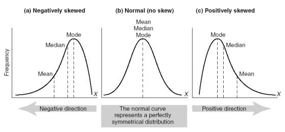
Skewness is lack of symmetry in a distribution of data.
[Technical note: we will be talking about skewness here in the context of unimodal distributions.]

A positive-skewed distribution means the right side tail of the distribution is longer or fatter than the left.
Likewise a negative-skewed distribution means the left side tail is longer or fatter than the right.
Symmetric distributions have no skewness!
Skewness and measures of central tendency
The mean, median, and mode are affected by skewness.
When a distribution is symmetrical, the mean, median, and mode are the same number.
When a distribution is negatively skewed, the mean is less than the median, which is less than the mode.
Negative skew: mean < median < mode
When a distribution is positively skewed, the mean is greater than the median, which is greater than the mode!
Positive skew: mode < median < mean
This way of thinking can help you, especially if you can't see a line graph of the data. All you need are the mean and the median. Nice!
- If the mean < median, the data are skewed left.
- If the mean > median, the data are skewed right.
Check: Using this information, does the list of numbers form a symmetric distribution? Is it skewed left of right?
Guided Practice: Range, Variance and Standard Deviation (20 mins)
Measures of variability like the range, variance, and standard deviation tell you about the spread of your data.
These measurements give complementary (and no less important!) information to the measures of central tendency (mean, median, mode).
Range
The range is the difference between the lowest and highest values of a distribution.
**calculate the range**
```python n = [3, 75, 98, 2, 10, 3, 14, 99, 44, 25, 31, 100, 356, 4, 23, 55, 327, 64, 6, 20] # In pure python: n = sorted(n) n_range = n[len(n) - 1] - n[0] print(n_range) 354 # With numpy: n_range = np.ptp(n) print(n_range) 354 ```Variance
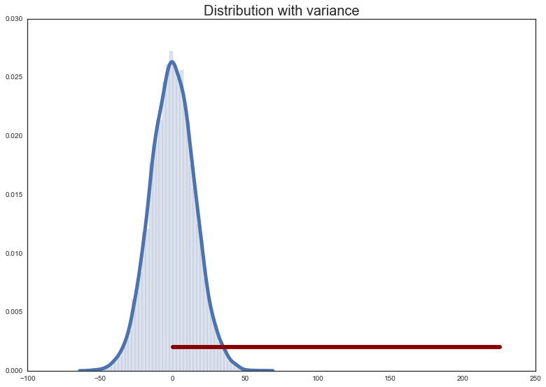
The variance is a numeric value used to describe how widely the numbers distribution vary.
In python variance can be calculated with:
variance = []
n_mean = np.mean(n)

for n_ in n:
  variance.append((n_ - n_mean) ** 2)

variance = np.sum(variance)
variance = variance / len(n)
Which is the average of the sum of the squared distances of each number from the mean of the numbers.

Check: What could a distribution with a large variance look like? A small?
Check: What does a variance of 0 mean?
Using numpy the variance is simply:
variance = np.var(n)

print(variance)
9414.6475
Standard deviation
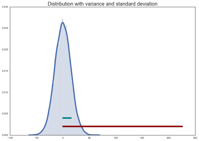
The standard deviation is the square root of the variance.
Because the variance is the average of the distances from the mean squared, the standard deviation tells us approximately, on average, the distance of numbers in a distribution from the mean.
The standard deviation can be calculated with:
std = np.std(n)

print(std)
97.029106457804716

Check: Is this the same as the average of the absolute deviations from the mean? If not, what is the difference between the measures?
Independent Practice: Topic (20 minutes)
- With the provided data, determine the mean, median, and mode.
- Is the data skewed left or right? How do you know?
- Find the range, variance and standard deviation of your data set. What does the standard deviation tell you about the distribution?
- Challenge: calculate the mode without using scipy!
Conclusion (5 mins)
- Review & recap
- Q & A