 Intro to Classification and Regression Trees (CARTs)
Week 6 | Lesson 1.1
LEARNING OBJECTIVES
After this lesson, you will be able to:
- Describe what a decision tree is
- Explain how a classification tree works
- Explain how a regression tree works
STUDENT PRE-WORK
Before this lesson, you should already be able to:
- Perform linear and polynomial regression
- Perform classification with KNN and Logistic Regression
- Use Python and Pandas to munge data
INSTRUCTOR PREP
Before this lesson, instructors will need to:
- Read in / Review any dataset(s) & starter/solution code
- Generate a brief slide deck
- Prepare any specific materials
- Provide students with additional resources
- Make sure that students have installed graphviz to visualize trees
LESSON GUIDE
| TIMING | TYPE | TOPIC |
|---|---|---|
| 5 mins | Opening | Opening |
| 45 min | Introduction | Intro to Classification and Regression Trees |
| 10 mins | Discussion | Discussion: The ID3 Algorithm for decision trees |
| 10 mins | Guided-practice | Guided Practice: Decision trees pros and cons |
| 10 mins | Ind-practice | Independent Practice: Decision trees as a service |
| 5 mins | Conclusion | Conclusion |
Opening (5 mins)
Last week we learned many new things.
Check: What were the most interesting things you learned last week? What were the hardest?
Answer: Hopefully they'll come up with things like: SQL, Postgres, SQLite, Pipelines, SVMs ...
This week we will learn about decision trees and ensemble methods. These are very powerful machine learning tools that allow us to solve complex problems in a very performant way. Also, they are easy to visualize and communicate, making them extremely powerful in a context where other (non-technical) stakeholders are involved.
Check: What do you already know about decision trees? What do you expect to learn?
Builds anticipation, stimulates thinking...
Intro to Decision Trees (25 min)
What a Decision Tree is
Decision trees are a non-parametric hierarchical classification technique.
- non-parametric means that the model is not described in terms of parameters like for example Logistic Regression. It also means that there is no underlying assumption on the distribution of data and of the error. In a sense this makes DT agnostic to the data.
- hierarchical means that the model consists of a sequence of questions which yield a class label when applied to any record. In other words, once trained, the model behaves like a recipe, which will tell us a result if followed exactly.
Consider the following example. Suppose I have a dataset of weather data, with 3 features: Outlook, Humidity, Wind, and a binary target variable which indicates if I should play golf on that day or not, depending on the weather. I could build a hierarchical tree of decisions like this one:
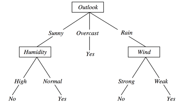
The tree gives me a precise rule to make a decision depending on the values assumed by the features.
Check: According to this tree, should I play golf in a day where:
- Outlook = Sunny
- Humidity = High
- Wind = Strong
Answer: No
Let's learn a little vocabulary. The tree is a case of Directed Acyclical Graph (DAG), and as such it has Nodes and Edges. Nodes correspond to questions or decisions, while edges correspond to possible answers to a given question.
The top node is also called root node it has 0 incoming edges, and 2+ outgoing edges. Internal nodes test a condition on a specific feature. They have 1 incoming edge, and 2+ outgoing edges. Finally a leaf node contains a class label (or a regression value). It has 1 incoming edge and 0 outgoing edges.
How to build a decision tree
In order to build a decision tree we need an algorithm that is capable of determining optimal choices for each node. One such algorithm is Hunt's algorithm: a greedy recursive algorithm that leads to a local optimum.
- greedy: algorithm makes locally optimal decision at each step
- recursive: splits task into subtasks, solves each the same way
- local optimum: solution for a given neighborhood of points
The algorithm works by recursively partitioning records into smaller and smaller subsets. The partitioning decision is made at each node according to a metric called purity. A node is said to be 100% pure when all of its records belong to a single class (or have the same value).
Example: binary classification with classes A, B
Given a set of records Dt at node t:
- If all records in
Dtbelong to class A, thentis a leaf node corresponding to class (Base case) - If
Dtcontains records from both A and B do the following:- create test condition to partition the records further
tis an internal node, with outgoing edges to child nodes- partition records in Dt to children according to test
These steps are then recursively applied to each child node.
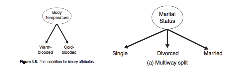
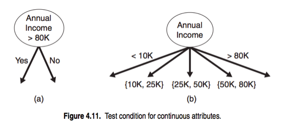
Splits can be 2 way or multi-way. Features can be categorical or continuous.
Check: Find rules to split the data below
| Exercises Completed | Total Time (min) | Result |
|---|---|---|
| 3 | 30 | Pass |
| 2 | 25 | Pass |
| 4 | 49 | Pass |
| 3 | 47 | Fail |
| 2 | 50 | Fail |
| 1 | 32 | Fail |
| 3 | 26 | Pass |
Optimization functions
Recall from the algorithm above, that we iteratively create test conditions to split the data. How do we determine the best split among all possible splits? Recall that no split is necessary (at a given node) when all records belong to the same class. Therefore we want each step to create the partition with the highest possible purity.
In order to do this, we will need an objective function to optimize. We want our objective function to measure the gain in purity from a particular split. Therefore we want it to depend on the class distribution over the nodes (before and after the split). For example, let $p(i|t)$ be the probability of class $i$ at node $t$ (eg, the fraction of records labeled $i$ at node $t$). Then for a binary (0/1) classification problem:
The maximum impurity partition is given by the distribution:
$$ p(0|t) = p(1|t) = 0.5
$$
where both classes are present in equal manner.
On the other hand, the minimum impurity partition is obtained when only one class is present, i.e:
$$ p(0|t) = 1 – p(1|t) = 1
$$
Therefore in the case of a binary classification we need to define an impurity function that will smoothly vary between the two extreme cases of minimum impurity (one class or the other only) and the maximum impurity case of equal mix.
We can define several functions that satisfy these properties. Here are three common ones:
$$ \text{Entropy}(t) = - \sum_{i=0}^{c-1} p(i|t)log_2 p(i|t)
$$
$$ \text{Gini}(t) = 1 - \sum_{i=0}^{c-1} [p(i|t)]^2
$$
$$ \text{Classification error}(t) = 1 - \max_i[p(i|t)]
$$
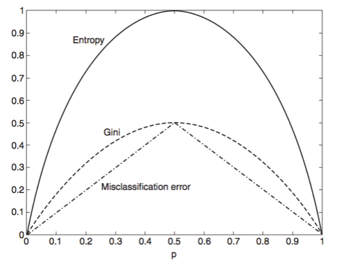
Note that each measure achieves its max at 0.5, min at 0 and 1.
Impurity measures put us on the right track, but on their own they are not enough to tell us how our split will do. We still need to look at impurity before & after the split. We can make this comparison using the gain:
$$ \Delta = I(\text{parent}) - \sum_{\text{children}}\frac{N_j}{N}I(\text{child}_j)
$$
Where $I$ is the impurity measure, $Nj$ denotes the number of records at child node $j$, and $N$ denotes the number of records at the parent node. When $I$ is the entropy, this quantity is called the _information gain.
Generally speaking, a test condition with a high number of outcomes can lead to overfitting (ex: a split with one outcome per record). One way of dealing with this is to restrict the algorithm to binary splits only (CART). Another way is to use a splitting criterion which explicitly penalizes the number of outcomes (C4.5).
Check: what properties does an impurity measure need to satisfy?
Answer:
- be zero when a class is pure
- be maximal when equal mixing
Discussion: The ID3 Algorithm for decision trees (15 mins)
Here's the pseudo code for the ID3 decision tree algorithm:
ID3 (Examples, Target_Attribute, Candidate_Attributes)
    Create a Root node for the tree
    If all examples have the same value of the Target_Attribute,
        Return the single-node tree Root with label = that value
    If the list of Candidate_Attributes is empty,
        Return the single node tree Root,
            with label = most common value of Target_Attribute in the examples.
    Otherwise Begin
        A ← The Attribute that best classifies examples (most information gain)
        Decision Tree attribute for Root = A.
        For each possible value, v_i, of A,
            Add a new tree branch below Root, corresponding to the test A = v_i.
            Let Examples(v_i) be the subset of examples that have the value v_i for A
            If Examples(v_i) is empty,
                Below this new branch add a leaf node
                    with label = most common target value in the examples
            Else
                Below this new branch add the subtree
                    ID3 (Examples(v_i), Target_Attribute, Attributes – {A})
    End
    Return Root
Let's go through it together. How would you implement that in python? Which data structure would you use?
Answer:
Decision Trees part 2 (15 min)
Check: What is overfitting? Why do we want to avoid it?
Answer: Overfitting occurs when a statistical model describes random error or noise instead of the underlying relationship. Overfitting generally occurs when a model is excessively complex, such as having too many parameters relative to the number of observations. A model that has been overfit will generally have poor predictive performance, as it can exaggerate minor fluctuations in the data.
Preventing overfitting
In addition to determining splits, we also need a stopping criterion to tell us when we’re done. For example, we can stop when all records belong to the same class, or when all records have the same attributes. This is correct in principle, but would likely lead to overfitting. One possibility is pre-pruning, which involves setting a minimum threshold on the gain, and stopping when no split achieves a gain above this threshold. This prevents overfitting, but is difficult to calibrate in practice (may preserve bias!). Alternatively we could build the full tree, and then perform pruning as a post-processing step. To prune a tree, we examine the nodes from the bottom-up and simplify pieces of the tree (according to some criteria). Complicated subtrees can be replaced either with a single node, or with a simpler (child) subtree. The first approach is called subtree replacement, and the second is subtree raising.
Decision tree regression
In the case of regression, the outcome variable is not a category but a continuous value. We cannot therefore use the same measure of purity we used for classification. Instead we will use the following variation of the algorithm:
At each node calculate the variance of the data points at that node, then choose the split that generates the largest decrease in total variance for the children nodes. In other words we use variance as our measure of impurity and we want to maximize the decrease of total variance at each split.
In a regression tree the idea is this: since the target variable does not have classes, we fit a regression model to the target variable using each of the independent variables. Then for each independent variable, the data is split at several split points. At each split point, the "error" between the predicted value and the actual values is squared to get a sum of squared errors (SSE). The split point errors across the variables are compared and the variable/point yielding the lowest SSE is chosen as the root node/split point. This process is recursively continued.
Guided Practice: Decision trees pros and cons (10 mins)
What do you think are the main advantages / disadvantages of decision trees? Discuss in pairs and then let's share.
Answer (from wikipedia):
- Advantages:
- Simple to understand and interpret. People are able to understand decision tree models after a brief explanation. => useful to work with non technical departments (marketing/sales).
- Requires little data preparation. Other techniques often require data normalization, dummy variables need to be created and blank values to be removed.
- Able to handle both numerical and categorical data. Other techniques are usually specialized in analyzing datasets that have only one type of variable.
- Uses a white box model. If a given situation is observable in a model the explanation for the condition is easily explained by boolean logic. By contrast, in a black box model, the explanation for the results is typically difficult to understand, for example with an artificial neural network.
- Possible to validate a model using statistical tests. That makes it possible to account for the reliability of the model.
- Robust. Performs well even if its assumptions are somewhat violated by the true model from which the data were generated.
- Performs well with large datasets. Large amounts of data can be analyzed using standard computing resources in reasonable time.
- Once trained can be implemented on hardware => extremely fast execution (real-time applications like trading or automotive).
- Disadvantages:
- Locally-optimal: The problem of learning an optimal decision tree is known to be NP-complete under several aspects of optimality and even for simple concepts. Consequently, practical decision-tree learning algorithms are based on heuristics such as the greedy algorithm where locally-optimal decisions are made at each node. Such algorithms cannot guarantee to return the globally-optimal decision tree. To reduce the greedy effect of local-optimality some methods such as the dual information distance (DID) tree were proposed.
- Overfitting: Decision-tree learners can create over-complex trees that do not generalize well from the training data. (use pruning to limit)
- There are concepts that are hard to learn because decision trees do not express them easily, such as XOR, parity or multiplexer problems. In such cases, the decision tree becomes prohibitively large.
Independent Practice: Decision trees as a service (10 mins)
There are several companies that offer decision trees as service. Two famous ones are BigML and WiseIO. Let's split the class in 2. One half will look at BigML case studies and the other half will look at WiseIO case studies.
Review a few of them with your team mates and choose one that you find particularly interesting. Then present it to the other group.
Conclusion (5 mins)
In this class we learned about Classification and Regression trees. We learned how Hunt's algorithm helps us recursively partition our data and how impurity gain is useful for determining optimal splits.
We've also reviewed the pros and cons of decision trees and industry
applications. In the next class we will learn to use them in Scikit-learn.