 Ensemble Methods - Random Forests and Boosting
Week 6| Lesson 3.1
LEARNING OBJECTIVES
After this lesson, you will be able to:
- Explain what a Random Forest is and how it is different from Bagging of Decision trees
- Explain what Extra Trees models are
- Apply both techniques to classification
- Describe Boosting and how it differs from Bagging
- Apply Adaboost and Gradient Boosting to classification problems
STUDENT PRE-WORK
Before this lesson, you should already be able to:
- Perform a classification using decision trees
- Describe how bagging works and use it in scikit learn
INSTRUCTOR PREP
Before this lesson, instructors will need to:
- Read in / Review any dataset(s) & starter/solution code
- Generate a brief slide deck
- Prepare any specific materials
- Provide students with additional resources
LESSON GUIDE
| TIMING | TYPE | TOPIC |
|---|---|---|
| 5 min | Opening | Opening |
| 25 min | Introduction | Intro to Random Forest |
| 20 min | Guided-practice | Guided Practice: Random Forest and ExtraTrees in Scikit Learn |
| 15 min | Introduction | Intro to Boosting |
| 15 min | Ind-practice | Independent Practice: Ada Boost and Gradient Boosting Classifier |
| 5 min | Conclusion | Conclusion |
Opening (5 mins)
Check: What happens when you combine bagging with decision trees? Recall some observations from the past labs and lessons.
Answer: generally performance improves
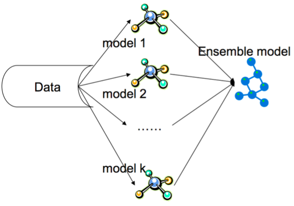
Today we will learn about random forests, which are essentially a variation of the bagging + decision tree model. We will also learn about a different ensemble technique called boosting and we will compare it with bagging.
Intro to Random Forest (25 min)
Random Forests are some of the most widespread classifiers used. They are relatively simple to use because they require very few parameters to set and they perform pretty well. As we have seen, Decision Trees are very powerful machine learning models.
Check: What are the main advantages of decision trees?
Answer:
- fast
- non parametric
- scale independent
- ...
On the other hand Decision Trees have some limitations, in particular, trees that are grown very deep tend to learn highly irregular patterns: they overfit their training sets. Bagging helps mitigate this problem by exposing different trees to different sub-samples of the whole training set.
Random forests are a further way of averaging multiple deep decision trees, trained on different parts of the same training set, with the goal of reducing the variance. This comes at the expense of a small increase in the bias and some loss of interpretability, but generally greatly boosts the performance of the final model.

Check: Describe how the bagging algorithm works:
Answer:
- sub sample with replacement
- train base models on subsamples
- combine prediction by average or majority vote
Random forests differ from bagging decision trees in only one way: they use a modified tree learning algorithm that selects, at each candidate split in the learning process, a random subset of the features. This process is sometimes called feature bagging. The reason for doing this is the correlation of the trees in an ordinary bootstrap sample: if one or a few features are very strong predictors for the response variable (target output), these features will be selected in many of the bagging base trees, causing them to become correlated. By selecting a random subset of the features at each split, we counter this correlation between base trees, strengthening the overall model.
Check: Recall what are the two properties base models must satisfy in order for bagging to work well.
Answer: base models must be:
- accurate: better than random guessing
- diverse: uncorrelated between one another
Typically, for a classification problem with $p$ features, $\sqrt{p}$ (rounded down) features are used in each split. For regression problems the inventors recommend $p/3$ (rounded down) with a minimum node size of 5 as the default.
Extremely Randomized Trees
Adding one further step of randomization yields extremely randomized trees, or ExtraTrees. These are trained using bagging and the random subspace method, like in an ordinary random forest, but an additional layer of randomness is introduced. Instead of computing the locally optimal feature/split combination (based on, e.g., information gain or the Gini impurity), for each feature under consideration, a random value is selected for the split. This value is selected from the feature's empirical range (in the tree's training set, i.e., the bootstrap sample), in other words, the top-down splitting in the tree learner is randomized.
Guided Practice: Random Forest and ExtraTrees in Scikit Learn (20 min)
Scikit Learn implements both random forest and extra trees methods as part of the ensemble module.
First have a look at the documentation. (5 min).
Check: What parameters did you notice? Any questions on those?
Let's load the car dataset.
import pandas as pd
df = pd.read_csv('./assets/datasets/car.csv')
df.head()
| buying | maint | doors | persons | lug_boot | safety | acceptability | |
|---|---|---|---|---|---|---|---|
| 0 | vhigh | vhigh | 2 | 2 | small | low | unacc |
| 1 | vhigh | vhigh | 2 | 2 | small | med | unacc |
| 2 | vhigh | vhigh | 2 | 2 | small | high | unacc |
| 3 | vhigh | vhigh | 2 | 2 | med | low | unacc |
| 4 | vhigh | vhigh | 2 | 2 | med | med | unacc |
This time we will encode the features using a One Hot encoding scheme, i.e. we will consider them as categorical variables. We also need to encode the label using the LabelEncoder.
from sklearn.preprocessing import LabelEncoder
y = LabelEncoder().fit_transform(df['acceptability'])
X = pd.get_dummies(df.drop('acceptability', axis=1))
We would like to compare the performance of the following 4 algorithms:
- Decision Trees
- Bagging + Decision Trees
- Random Forest
- Extra Trees
Note that in order for our results to be consistent we have to expose the models to exactly the same Cross Validation scheme. Let's start by initializing that.
from sklearn.cross_validation import cross_val_score, StratifiedKFold
from sklearn.tree import DecisionTreeClassifier
from sklearn.ensemble import RandomForestClassifier, ExtraTreesClassifier, BaggingClassifier

cv = StratifiedKFold(y, n_folds=3, shuffle=True, random_state=41)
Now let's initialize a Decision Tree Classifier and evaluate its performance:
dt = DecisionTreeClassifier(class_weight='balanced')
s = cross_val_score(dt, X, y, cv=cv, n_jobs=-1)
print "{} Score:\t{:0.3} ± {:0.3}".format("Decision Tree", s.mean().round(3), s.std().round(3))
Decision Tree Score: 0.962 ± 0.008
Your turn now:
Initialize the following models and check their performance:
- Bagging + Decision Trees
- Random Forest
- Extra Trees
You can also create a function to speed up your work...
Answer:
bdt = BaggingClassifier(DecisionTreeClassifier())
rf = RandomForestClassifier(class_weight='balanced', n_jobs=-1)
et = ExtraTreesClassifier(class_weight='balanced', n_jobs=-1)

def score(model, name):
    s = cross_val_score(model, X, y, cv=cv, n_jobs=-1)
    print "{} Score:\t{:0.3} ± {:0.3}".format(name, s.mean().round(3), s.std().round(3))

score(dt, "Decision Tree")
score(bdt, "Bagging DT")
score(rf, "Random Forest")
score(et, "Extra Trees")

Decision Tree Score:    0.962 ± 0.008
Bagging DT Score:    0.966 ± 0.004
Random Forest Score:    0.948 ± 0.009
Extra Trees Score:    0.955 ± 0.004
In this case the Bagging Decision tree seems to still be performing better than the other models, although the scores are compatible within the error. With other datasets the Random Forest and the Extra Trees model could be performing better and thus are worth testing.
Intro to Boosting (15 min)
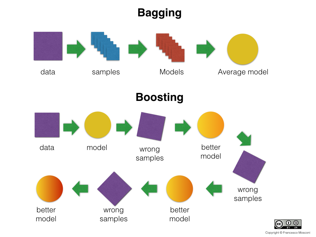
With bagging and random forests we train models on separate subsets and then combine their prediction. In a sense we are parallelizing the training and then combining (like a map-reduce).
Boosting is a different ensemble technique that is sequential.

Boosting is an iterative procedure that adaptively changes the sampling distribution of training records at each iteration in order to correct the errors of the previous iteration of models. The first iteration uses uniform weights (like bagging) for all samples. In subsequent iterations, the weights are adjusted to emphasize records that were misclassified in previous iterations. The final prediction is constructed by a weighted vote (where the weights for a base classifier depends on its training error).
Since the base classifier's focus more and more closely on records that are difficult to classify as the sequence of iterations progresses, they are faced with progressively more difficult learning problems.
Boosting takes a base weak learner and tries to make it a strong learner by re-training it on the misclassified samples.
There are several algorithms for boosting, in particular we will mention AdaBoost, GradientBoostingClassifier that are implemented in scikit learn.
AdaBoost
AdaBoost refers to a particular method of training a boosted classifier. A boost classifier is a classifier in the for
$$ FT(x) = \sum{t=1}^T f_t(x)
$$ where each $f_t$ is a weak learner that takes an object $x$ as input and returns a real valued result indicating the class of the object.
Each weak learner produces an output, hypothesis $h(x_i)$, for each sample in the training set. At each iteration $t$, a weak learner is selected and assigned a coefficient $\alpha_t$ such that the sum training error $E_t$ of the resulting t-stage boost classifier is minimized.
$$ Et = \sum_i E[F{t-1}(x_i) + \alpha_t h(x_i)]
$$
Here $F_{t-1}(x)$ is the boosted classifier that has been built up to the previous stage of training, $E(F)$ is some error function and $f_t(x) = \alpha_t h(x)$ is the weak learner that is being considered for addition to the final classifier.
At each iteration of the training process, a weight is assigned to each sample in the training set equal to the current error $E(F_{t-1}(x_i))$ on that sample. These weights can be used to inform the training of the weak learner, for instance, decision trees can be grown that favor splitting sets of samples with high weights.
Gradient Boosting Classifier
Gradient Boosting is a generalization of boosting to arbitrary differentiable loss functions. GBRT is an accurate and effective off-the-shelf procedure that can be used for both regression and classification problems. Gradient Tree Boosting models are used in a variety of areas including Web search ranking and ecology.
The advantages of GBRT are:
- Natural handling of data of mixed type (= heterogeneous features)
- Predictive power
- Robustness to outliers in output space (via robust loss functions)
The disadvantages of GBRT are:
- Scalability, due to the sequential nature of boosting it can hardly be parallelized.
Independent Practice: Ada Boost and Gradient Boosting Classifier (15 min)
Test the performance of the AdaBoost and GradientBoostingClassifier models on the car dataset. Use the code you developed above as a starter code.
Solution:
    from sklearn.ensemble import AdaBoostClassifier, GradientBoostingClassifier
    ab = AdaBoostClassifier()
    gb = GradientBoostingClassifier()
    score(ab, "AdaBoost")
    score(gb, "Gradient Boosting Classifier")
    # AdaBoost Score:    0.811 ± 0.002
    # GBoost Score:    0.982 ± 0.006
Conclusion (5 min)
In this class we learned about Random Forest, Extremely randomized trees and Boosting. They are different ways to improve the performance of a weak learner.
Some of these methods will perform better in some cases, some better in other cases. For example, Decision Trees are more nimble and easier to communicate, but have a tendency to overfit. On the other hand Ensemble methods perform better in more complex scenarios, but may become very complicated and harder to explain. Have a look here for a couple of examples from real world startup Wise.io.
Check: Can you think of what could be limitations of these methods?
Answer:
- They don't scale very well to large datasets, Boosting in particular
- They are black boxes