 Bias Variance Tradeoff
Week 3 | Lesson 2.1
LEARNING OBJECTIVES
After this lesson, you will be able to:
- Define bias and variance intuitively
- Explain models error in terms of bias and variance
STUDENT PRE-WORK
Before this lesson, you should already be able to:
- Fit linear models
- Understand the sum of squared errors calculation (SSE).
INSTRUCTOR PREP
Before this lesson, instructors will need to:
- Read in / Review any dataset(s) & starter/solution code
- Generate a brief slide deck
- Prepare any specific materials
- Provide students with additional resources
STARTER CODE
LESSON GUIDE
| TIMING | TYPE | TOPIC |
|---|---|---|
| 5 min | Opening | Opening |
| 10 min | Introduction | Bias-Variance Tradeoff |
| 15 min | Demo | Examples of Bias and Variance |
| 25 min | Guided Practice | Explore Bias and Variance |
| 25 min | Independent Practice | Explore Bias and Variance |
| 5 min | Conclusion | Conclusion |
Opening (5 mins)
- Review prior labs/homework, upcoming projects, or exit tickets, when applicable
- Review lesson objectives
- Discuss real world relevance of these topics
- Relate topics to the Data Science Workflow - i.e. are these concepts typically used to acquire, parse, clean, mine, refine, model, present, or deploy?
Check: Ask students to define, explain, or recall any relevant prework concepts.
Introduction: Bias-Variance Tradeoff (20 mins)
This is a more complicated topic than the previous lessons and you will likely spend more time lecturing. Try to make good use of the included instructor plot notebook whenever you need to run the plots described in this lesson, and spend more time in the demo notebook as needed.
Now that we're getting better at finding and fitting linear models, it's time to learn how to analyze how well our models actually fit the data, and how we can make good choices and better models. Usually we attempt to quantify the error in our models, the difference between predictions and true values, and we'll learn multiple ways to do so. We've already seen one such measure, the sum of the squared errors (SSE).
SSE is commonly decomposed into bias and variance. Conceptually, a model is biased if it makes assumptions about what the data should look like and misses the mark. For example, a line is not a good global approximation for a parabola:
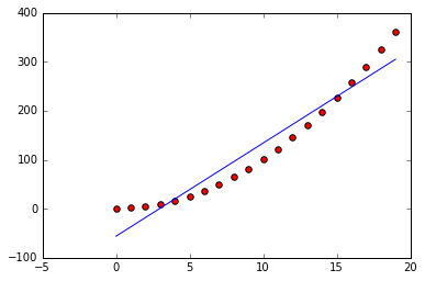
In this case our model has an opinion about the shape of the data that's not quite right, so we say it is biased. More data isn't going to help, and a different sampling of data won't either. Our model is simply biased and won't ever be a good fit to the data.
Let's see how to calculate the bias so that we can make this idea precise.
We describe our model as a relationship between our data's observables x_i, our targets y_i (the true values), and some inherent noise e, usually assumed to be normally-distributed with mean zero and variance \sigma^2. Then our model is described by a function f as:
y_i = f(x_i) + e_i
The function f(x) = a x + b describes the linear models that we've been working with so far this week. As modelers, our goal is to find the function F that minimizes our error.
To describe the bias in a given model F, we look at the difference between the average prediction of our model and the true values. Our attempt to fit a linear model to a parabola above has a lot of bias because the average difference between our model's predictions and the true values is large (even though some points are accurately predicted). By average we mean over many attempts at the modeling process -- if we repeat the modeling process with more samples of data from the same source with the same type of model, we'll find similar amounts of error on average due to our mismatch in model assumptions and the data's true distribution.
If we tried to fit a model like y=a x + b x^2 + e to our parabolic model, we could find a model with much less bias (on average):
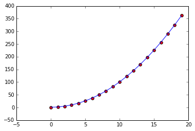
On the other hand if we had tried a cubic model without a quadratic or linear term, i.e. y = a x^3 + b1, we'd still have a lot of bias (on average):
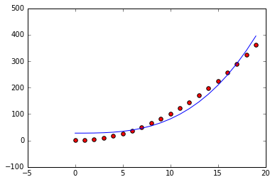
Usually there is a sweet spot where the bias is low and the model is the right complexity. You might think that we can always use a high degree polynomial with lots of parameters to find a low bias model, and that's somewhat true. The unnecessary parameters will be fit close to zero and our model will generally have low bias if the data is polynomial in nature. But it turns out there is another source of error from using models with many parameters.
Since our data has inherent errors, small fluctuations in the data can introduce artifacts that our model will attempt to fit. If we have a lot of parameters, we may end up fitting a model that doesn't fit the data, or doesn't well fit another sample of data from the same source. For example, with the following data points we could try to fit a line or a higher dimensional polynomial:
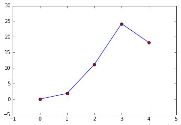
The polynomial fits nearly perfectly but the underlying data may not actually come from such a shape. If we take data from the same source and repeat the fit:
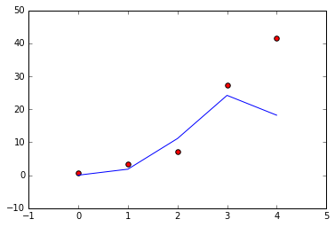
In this case the model we fit on the first sample overfit the data and doesn't fit the second sample well even though they are from the same source. We call this source of error the error due to variance.
Check: We've described two sources of error:
- bias
- variance What is the difference between them?
There is a nice Visualization that is similar to the relationship between precision and accuracy
The Tradeoff
There is a third source of error, the error inherent in our model. This is the
error term e which has variance \sigma^2. Combining all these sources of
data gives us the squared error:

This equation is why bias and variance are often described as a tradeoff. However it's more accurate to describe the relationship with an plot:
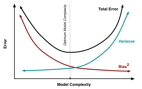
As you can see there is usually a sweet spot in "model space" where bias and variance are both small, so low variance doesn't necessarily imply high bias. Note too that there's nothing we can do to reduce the inherent noise in the data. The tradeoff is in the rates of bias and variance as a function of model complexity.
Demo: Examples of Bias and Variance (15 mins)
Use the included demo notebook to demo a series of models and explore both the bias and the variance.
Emphasize that bias and variance are properties that arise over many data samples and model fits.
Guided Practice: Explore Bias and Variance (20-30 mins)
We've seen that as the complexity in our models change so too do the bias and variance. Let's investigate from another angle using linear regression. Rather than change the model, we'll change the underlying data to be drawn from a higher dimensional model.
Your tasks are:
- Fill in the code to fit a linear regression to the data
- investigate the bias and variance as the data source changes in complexity
Get started with the Starter Code!
Check student work with these solutions
Independent Practice: Explore Bias and Variance (20-25 minutes)
Now let's look at some situations where adding more polynomial terms decreases both bias and variance.
Get started with the Starter Code!
Check student work with these solutions
Conclusion (5-10 mins)
There are three fundamental sources of error that arise when fitting a model to data:
- Bias
- Variance
- Inherent noise
We can't do much about the inherent noise in the data, but we can often reduce both bias and variance with good choices of models.