Support Vector Machines

Week 5 | Lesson 5.1

Note: This lesson is a bonus/optional component for Week 5. Feel free to swap this out for additional review & project work as needed.

LEARNING OBJECTIVES

After this lesson, you will be able to:

Describe what a Support Vector Machine (SVM) model is
Explain the math that powers it
Evaluate pros/cons compared to other models
Know how to tune it

STUDENT PRE-WORK

Before this lesson, you should already be able to:

Perform regression
Perform regularization

INSTRUCTOR PREP

Before this lesson, instructors will need to:

Read in / Review any dataset(s) & starter/solution code
Generate a brief slide deck
Prepare any specific materials
Provide students with additional resources

LESSON GUIDE

TIMING	TYPE	TOPIC
5 mins	Opening	Opening
45 mins	Introduction	Introduction: Support Vector Machines
10 mins	Demo	Demo: Linear SVM
20 mins	Guided-practice	Guided Practice: Tuning an SVM
5 mins	Conclusion	Conclusion

Opening (5 mins)

Today we will learn about Support Vector Machines.

Check: What do you think the name means?

Introduction: Support Vector Machines (45 mins)

A support vector machine (SVM) is a binary linear classifier whose decision boundary is explicitly constructed to minimize generalization error.

Recall:

Binary classifier – solves two-class problem
Linear classifier – creates linear decision boundary (in 2d)

The decision boundary is derived using geometric reasoning (as opposed to the algebraic reasoning we’ve used to derive other classifiers). The generalization error is equated with the geometric concept of margin, which is the region along the decision boundary that is free of data points.

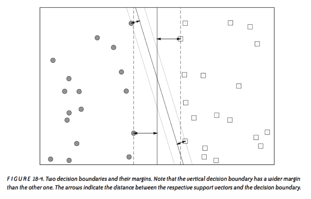
The goal of an SVM is to create the linear decision boundary with the largest margin. This is commonly called the maximum margin hyperplane (MMH).

Nonlinear applications of SVM rely on an implicit (nonlinear) mapping that sends vectors from the original feature space K into a higher-dimensional feature space K’. Nonlinear classification in K is then obtained by creating a linear decision boundary in K’. In practice, this involves no computations in the higher dimensional space, thanks to what is called the kernel trick.

Decision Boundary

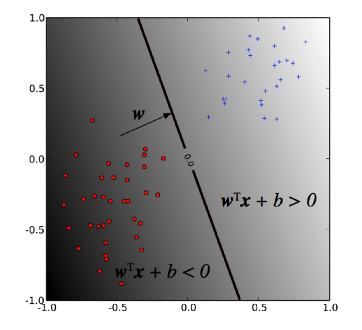
The decision boundary (MMH) is derived by the discriminant function:

$$ f(x) = w^T x + b

where w is the weight vector and b is the bias. The sign of f(x) determines the (binary) class label of a record x.

As we said before, SVM solves for the decision boundary that minimizes generalization error, or equivalently, that has the maximum margin. These are equivalent since using the MMH as the decision boundary minimizes the probability that a small perturbation in the position of a point produces a classification error.

Selecting the MMH is a straightforward exercise in analytic geometry (we won’t go through the details here). In particular, this task reduces to the optimization of the following convex objective function:

$$\text{minimize: } \space \frac{1}{2}||w||^2$$

$$\text{subject to: } y_i(w^T x_i + b) \geq 1 \text{ for } i = 1,..,N$$

Notice that the margin depends only on a subset of the training data; namely, those points that are nearest to the decision boundary.

These points are called the support vectors. The other points (far from the decision boundary) don’t affect the construction of the MMH at all.

This formulation only works if the two classes are linearly separable, so that we can indeed find a margin to separate them. Usually however, classes are not separable, and there is partial overlap between them. This requires an extension of the formulation to accommodate for class overlap.

Soft margin, slack variables

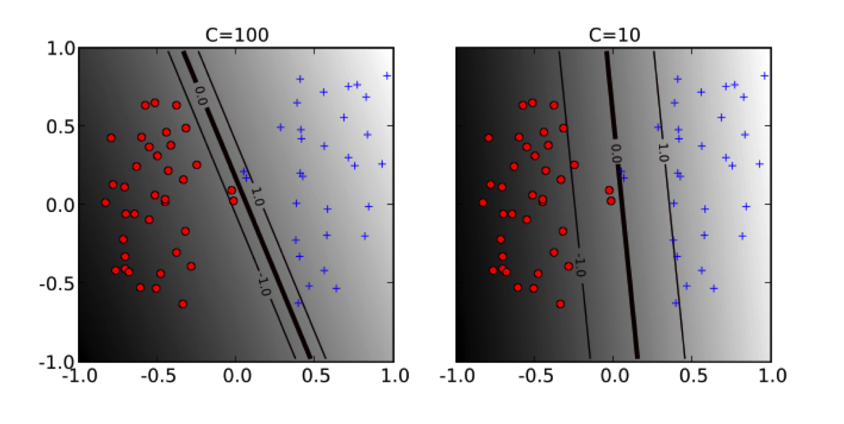
Class overlap is achieved by relaxing the minimization problem or softening the margin. This amounts to solving the following problem:

$$ \text{minimize: } \space \frac{1}{2}||w||^2 + C \sum_{i=1}^N \xi_i $$

$$ \text{subject to: } y_i(w^T x_i + b) \geq 1 - \xi_j \text{ for } i = 1,..,N \text{ and } \xi_i > 0 $$

The hyper-parameter C (soft-margin constant) controls the overall complexity by specifying penalty for training error. This is yet another example of regularization.

Nonlinear SVM

The soft-margin optimization problem can be rewritten as:

$$ \text{maximize: } \sum_{i=1}^N \alpha_i

\frac{1}{2}\sum{i=1}^N\sum{j=1}^N yi y_j \alpha_i \alpha_j x^Tx$$ $$ \text{subject to: } \sum{i=1} y_i \alpha_i = 0, 0 \leq \alpha_i \leq C $$

Since the feature vector $x$ only appears in the inner product, we can replace this inner product with a more general function that has the same type of output as the inner product. This is called kernel trick.

Formally, we can think of the inner product as a map that sends two vectors in the feature space K into the real line $R$. A kernel function is a non-linear map the sends two vectors in a higher-dimensional feature space K’ into the real line $R$.

See here for a deeper tutorial on the math.

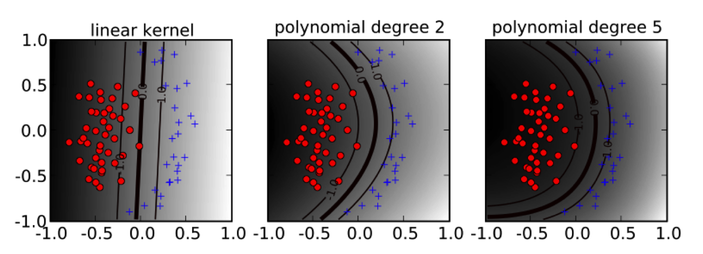
Some popular kernels

Linear kernel: $ k(x, x') = x^T x' $
Polynomial kernel: $ k(x, x') = (x^T x' + 1)^d$
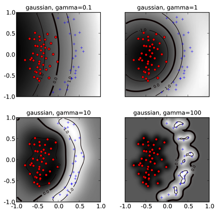
Gaussian kernel (rbf): $ k(x, x') = \exp{(-\gamma||x - x'||^2)} $

The hyperparameters $d$ and $\gamma$ affect the flexibility of the decision boundary.

Demo: Linear SVM (10 mins)

Scikit-learn implements support vector machine models in the svm package.

import pandas as pd
import numpy as np
from sklearn.svm import SVC
from sklearn.datasets import load_iris

iris = load_iris()

X = iris.data
y = iris.target

model = SVC(kernel='linear')
model.fit(X, y)

SVC(C=1.0, cache_size=200, class_weight=None, coef0=0.0,
  decision_function_shape=None, degree=3, gamma='auto', kernel='linear',
  max_iter=-1, probability=False, random_state=None, shrinking=True,
  tol=0.001, verbose=False)

Notice that the SVC class has several parameters. In particular we are concerned with two:

C: penalty parameter of the error term (regularization)
kernel: the type of kernel used (linear, poly, rbf, sigmoid, precomputed or a callable.)

Notes from the documentation:

In the current implementation the fit time complexity is more than quadratic with the number of samples which makes it hard to scale to dataset with more than a couple of 10000 samples.
The multi-class support is handled according to a one-vs-one scheme.

As usual we can calculate the cross validated score to judge the quality of the model.

from sklearn.cross_validation import cross_val_score

cvscores = cross_val_score(model, X, y, cv = 5, n_jobs=-1)
print "CV score: {:.3} +/- {:.3}".format(cvscores.mean(), cvscores.std())

CV score: 0.98 +/- 0.0163

Guided Practice: Tuning an SVM (20 minutes)

An SVM almost never works without tuning its parameter.

Check: Try performing a grid search over kernel type and regularization strength to find the optimal score for the above data.

Answer:

from sklearn.grid_search import GridSearchCV
parameters = {'kernel':('linear', 'rbf'), 'C':[0.1, 1, 3, 10]}
clf = GridSearchCV(model, parameters, n_jobs=-1)
clf.fit(X, y)
clf.best_estimator_

Check: Can you think of pros and cons for Support Vector Machines

Pros:

Very powerful, good performance

Can be used for anomaly detection (one-class SVM)

Cons:

Can get very hard to train with lots of data

Prone to overfit (need regularization)

Black box

Conclusion (5 mins)

In this class we have learned about Support Vector Machines. We've seen how they are powerful in many situations and what can some of their limitations be.

Can you think of a way to apply them in business?

5.1 Support Vector Machines