 Tuning the ARIMA Model
Week 9 | Lesson 4.1
LEARNING OBJECTIVES
After this lesson, you will be able to:
- Incorporate Seasonal factors in the ARIMA model
- Add Seasonal factors to your ARIMA model to tune the predictions
- Demonstrate the use of differencing in analysing Time Series data
STUDENT PRE-WORK
Before this lesson, you should already be able to:
- Train the ARIMA model
- Compute differences in Time Series data
- Analyse the output of ACF and PACF graphs to determine necessary transformations
INSTRUCTOR PREP
Before this lesson, instructors will need to:
- Read in / Review any dataset(s) & starter/solution code
- Generate a brief slide deck
- Prepare any specific materials
- Provide students with additional resources
- Read following note, decide student approach, prepare environment
STARTER CODE
IMPORTANT NOTE!
At the time of writing, SARIMAX is not included in the stable release of statsmodels. Students will need to install the development version of statsmodels (>= 0.7) in a conda env by entering the following commands in their terminal. Please do this at the beginning of class if you would like them to code along with you, or before they begin lab 4.2 if they will just be watching your live-coding.
conda create -n statsmodeldevenv python=2.7 pandas numpy scipy ipython jupyter patsy cython matplotlib
source activate statsmodeldevenv
git clone git://github.com/statsmodels/statsmodels.git
cd statsmodels/
python setup.py install
LESSON GUIDE
| TIMING | TYPE | TOPIC |
|---|---|---|
| 10 min | Opening | Opening |
| 15 min | Introduction | Seasonal ARIMA |
| 10 min | Discussion | ACF/PACF Usage |
| 15 min | Codealong | European Retail Trade Data EDA |
| 15 min | Codealong | European Retail Trade Data Modeling |
| 10 min | Introduction | The Ljung-Box Test |
| 25 min | Demo | Tuning SARIMA |
| 10 min | Codealong | Predictions |
| 10 min | Conclusion | Topic description |
Opening (10 mins)
Thus far we have investigated the Non-Seasonal ARIMA model. If you recall, at the end of our last lesson, we were stuck with a sub-optimal model. Can you recall exactly why we were unable to tune our parameters further?
Answer: The issue came down to seasonality, but more specifically:
- Increasing p would increase the dependency on previous values further (longer lag), but this isn't necessary past a given point.
- Increasing q would increase the dependency of an unexpected jump at a handful of points, but we did not observe that in our autocorrelation plot.
- Increasing d would increase differencing, but with d=1 we saw a move towards stationarity already (except at a few problematic regions). Increasing to 2 may be useful if we are saw an exponential trend, but that we did not here.
Now we will introduce the Seasonal ARIMA model to address the Seasonal elements of Time Series Data.
Before we begin, be sure to use the commands detailed above to install the dev package for statsmodels.
Introduction: Seasonal ARIMA (10 mins)
The Seasonal ARIMA model combines the Non-Seasonal ARIMA with Seasonal factors in a multiplicative model. This model assumes that as the data increase, so does the seasonal pattern. Most time series plots exhibit such a pattern. In this model, the trend and seasonal components are multiplied and then added to the error component.
The model is notated as follows:
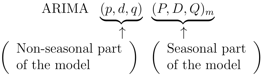
Let's take a look at each of the parameters:
- p = non-seasonal AR order
- d = non-seasonal differencing
- q = non-seasonal MA order
- P = seasonal AR order
- D = seasonal differencing
- Q = seasonal MA order
- m = number of periods per season
In identifying a seasonal model, the first step is to determine whether or not a seasonal difference is needed. We can do that by investigating the ACF and PACF graphs for our data.
Discussion: ACF/PACF Usage (10 mins)
Instructor's Note: It will be helpful to use the whiteboard to draw ACF/PACF patterns that correspond with this lesson
We can determine the seasonal parameters for an AR or MA model using the seasonal lags that appear in the ACF and PACF. For example, an ARIMA(0,0,0)(0,0,1)12 model would have the following characteristics:
- A spike at k = 12 in the ACF, but no other significant spikes
- Exponential decay in seasonal lags in the PACF (i.e. decay at lags 12, 24, 36, ...)
By observing these characteristics, we would have deduced that m = 12, and our seasonal MA order should be 1.
CHECK: Calling on the information gained in the last lesson, why does this make sense?
Similarly, an ARIMA(0,0,0)(1,0,0)12 model would show the following:
- A spike at k = 12 in the PACF, but no other significant spikes
- Exponential decay in seasonal lags in the ACF
If the data you are investigating displays a seasonal pattern that is both strong and stable over time (i.e. temperatures are higher in the Summer, lower in the Winter), then it is likely that your Seasonal Difference term D should be set to 1. This will prevent the seasonal pattern from "dying out" in the long-term forecasts.
NOTE: NEVER use more than ONE order of Seasonal Differencing, or more than 2 orders of total differencing (Seasonal + Non-Seasonal).
In considering the appropriate seasonal orders for an ARIMA model, focus solely on the seasonal lags. The modeling procedure is almost the same as for non-seasonal data, except that we need to select seasonal AR and MA terms as well as the non-seasonal components of the model. This process can be best illustrated using examples, so let's walk through one now.
Codealong: European Retail Trade Data EDA (15 mins)
Let's take a look at this data set, which displays European retail trade data reported quarterly from 1996-2011. To start, let's load the data into pandas and build a basic plot.
import pandas as pd
%matplotlib inline

df = pd.read_csv('../../assets/data/euretail.csv')
df = df.set_index(['Year'])
df.stack().plot()

Off the bat, what can we tell about our data? We see that our data is Non-Stationary, and there are some apparent seasonal patterns. Let's take a Seasonal Difference to see what effect that has. What should our value for m be in this case?
Answer: Best to start with 4, because our samples are taken quarterly
from statsmodels.graphics.tsaplots import plot_acf, plot_pacf
diff0 = df.stack().diff(periods=4)[4:]
diff0.plot(title='European Retail Trade Differenced')
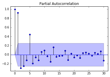
plot_acf(diff0, lags=30)
plot_pacf(diff0, lags=30)
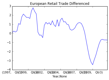

What does this tell us, and what should we do next?
Answer: The data is still non-stationary, so let's take an additional first order difference.
diff1 = diff0.diff()[1:]
diff1.plot(title='European Retail Trade Differenced Twice')
plot_acf(diff1, lags=30)
plot_pacf(diff1, lags=30)
Now we have stationary data, and have a good idea of which values for d and D we want for our model.
Codealong: European Retail Trade Data Modeling (15 mins)
The next step is to find appropriate AR, MA, Seasonal AR, and Seasonal MA terms for our model. We will do this using the ACF and PACF of the doubly difference data. Our ACF shows a significant spike at lags 1 and 4. The first spike suggests a non-seasonal MA(1) component, while the second spike suggests a seasonal MA(1) component.
Therefore, we will start with an ARIMA(0,1,1)(0,1,1)4 model.
CHECK: Make sure you understand the reasoning behind the choices made to populate all of the Seasonal ARIMA parameters. Can you explain each to the person sitting next to you?
import statsmodels.api as sm
data = df.stack().values
model = sm.tsa.statespace.SARIMAX(data, order=(0,1,1), seasonal_order=(0,1,1,4))
results = model.fit()
print results.summary()
Take a moment to inspect the results summary before plotting the residuals. As we've only auditioned one model, the summary won't tell us much, but what do you see? Let's go ahead and plot the residuals and their ACF/PACF.
# Don't plot the first 5 values, to account for data loss when differencing (d=1 + D=5)
residuals = results.resid[5:]
plt.plot(residuals)

plot_acf(residuals, lags=30)
plot_pacf(residuals, lags=30)
What do we see? There are significant spikes at lag 2 in both ACF and PACF, and an almost significant spike at lag 3. This indiactes that some additional non-seasonal terms are needed.
Instructor's Note: Now might be a good time to reinforce the difference between seasonal and non-seasonal terms, and how to detect which are necessary based on ACF/PACF readings
Introduction: The Ljung-Box Test (10 Mins)
The Ljung-Box test is a type of statistical test of whether any of a group of autocorrelations of a time series are different from zero. Instead of testing randomness at each distinct lag, it tests the “overall” randomness based on a number of lags. We can use this heuristic to test the fit of our model. By using the Ljung-Box test, we can determine whether the residuals from our model have any autocorrelation.
It is computed as such:
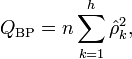
Statsmodels leaves it up to the user to select the number of lags. For time series that are Non-Seasonal, it is recommended that you use k = MIN(10, T/5). In other words, if your sample has over 50 observations, then your k should be the number of periods divided by 5. Otherwise, use k = 10.
Let's evaluate the output of the Ljung-Box test by checking the p-values, which are the second results provided. If the p-value is high, we will accept the Null Hypothesis that our data is Random.
from statsmodels.stats.diagnostic import acorr_ljungbox

lags = min(10, len(residuals)/5)

acorr_ljungbox(residuals, lags=lags)
What does the output tell us?
Answer: The p-value of 0.22 at lag k = 11 tells us that the residuals have no autocorrelations and are seemingly random
Guided Practice: Seasonal ARIMA Tuning (25 mins)
We're going to tune this further. On your own, or with a partner, start auditioning more SARIMA models on our data. Open the sarima.ipynb notebook to get started.
Some tips along the way:
- Record your AIC values for each SARIMA model
- Examine the ACF/PACF of your residuals. Do they resemble white noise?
- For each model you try, add a comment as to the effect you think your tuning had
- Try only altering one term at a time
Instructor's Note: After the guided practice, spend 5 minutes going over the results. The best course of action is to increment the Non-Seasonal AR term, and then extract the AIC. i.e.: ARIMA(0,1,2)(0,1,1)4 -> 73.618 AIC ARIMA(0,1,3)(0,1,1)4 -> 67.946 AIC (I found this to be the best fit)
Let's go ahead and review the models. Who found the lowest AIC? Let's discuss how you got there, and what you've learned.
Codealong: Predictions (10 mins)
Now that we've chosen a model, let's chart our predictions. We can use the built in forecast function to make this easy. Let's go over a quick way to view our forecast.
preds = res.forecast(12)
fcast = np.concatenate((data, preds), axis=0)

plt.figure();
plt.plot(data, 'o' , fcast, 'r--');
CHECK: Do these predictions look meaningful based on the data? How do the predictions compare to the Non-Seasonal ARIMA model?
Conclusion (10 mins)
Instructor's notes:
Review the subject covered in this lesson. Discuss key takeaways in tuning the ARIMA model by adding seasonal factors.
Explain that these models typically take months to tune. We are not expecting students to leave with a working knowledge of ARIMA/SARIMA models, but insights into the kind of work we do as Data Scientists.
Discuss the Kaggle project to make sure everyone is prepared for tomorrow's presentations!
UPCOMING ASSIGNMENTS
| HOMEWORK | Example Assignment | Session Due |
| PROJECTS | Project Title | Session Due |