 Autocorrelation & Time Series Data
Week 9 | Lesson 2.2
LEARNING OBJECTIVES
After this lesson, you will be able to:
- Be able to explain Autocorrelation from mathematical, technological and practical perspectives
- Perform Autocorrelation in Pandas
STUDENT PRE-WORK
Before this lesson, you should already be able to:
- Use Pandas to load, access and mutate time series data
- Plot data using Tableau (or another plotting utility)
INSTRUCTOR PREP
Before this lesson, instructors will need to:
- Review lab 2.1 - Analyzing Time Series Data
- Read through datasets and starter/solution code
- Add to the "Additional Resources" section for this lesson
STARTER CODE
LESSON GUIDE
| TIMING | TYPE | TOPIC |
|---|---|---|
| 5 min | Opening | Lesson Objectives |
| 15 min | Introduction | Trend and Seasonality |
| 65 min | Demo/Codealong | Autocorrelation |
| 5 min | Conclusion | Topic description |
Opening (5 mins)
- Review lab 2.1 - Analyzing Time Series Data
QUESITON: What are some real world scenarios where Time Series Data Analysis is useful?
Answer: Answers can include any of the following:
- Finance Planning
- Inventory Volume Analysis
- Climate Change
- Etc.
In this lesson, we will discuss statistics associated with data with that is changing over time and look at how to measure that change.
Specifically, we will focus on identifying problems that are related to time series data and then understanding the types of questions we are interested in. Additionally, we will discuss the unique aspects of mining and refining time series data.
Introduction: Trend and Seasonality (15 mins)
QUESTION: What constitutes a trend in data? Is Linearity required for Trend?
Answer:
- A trend exists when there is a long-term increase or decrease in the data.
- No
Trend may “change direction” when it goes from an increasing trend to a decreasing trend. Trend can only be measured in the scope of the data collected, though there may be trends that are unmeasureable if the data is not complete.
An example of an upward trend:
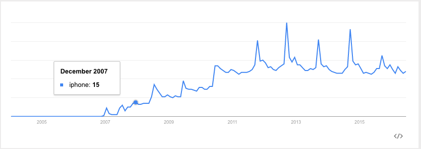
When there are patterns that repeat over known, fixed periods of time within the data set it is considered to be seasonality, seasonal variation, periodic variation, or periodic fluctuations- all different terms, but they mean the same thing. A seasonal pattern exists when a series is influenced by factors relating to the cyclic nature of time - i.e. time of month, quarter, year, etc. Seasonality is always of a fixed and known period, otherwise it is not truly seasonality, and must be either attributed to another factor or counted as a set of anomalous events in the data.
The easiest way to visualize trend is by drawing Trend Lines- a common practice in Excel. We'll show you how to do this in Python. Please open the trendlines ipython notebook for this demonstration.
Demo/Codealong: Autocorrelation (65 mins)
What is Autocorrelation?
While in previous weeks, our analyses has been concerned with the correlation between two or more variables (height and weight, education and salary, etc.), in time series data, autocorrelation is a measure of how correlated a variable is with itself. Specifically, autocorrelation measures how closely related earlier variables are with variables occurring later in time.
How do we compute Autocorrelation?
To compute autocorrelation, we fix a lag k which is the delta between the given point and the prior point used to compute the correlation.
With a k value of 1, we'd compute how correlated a value is with the prior one. With a k value of 10, we'd compute how correlated a variable is with one 10 time points earlier.
Check: Assert that the students are able to explain what Autocorrelation is and how it works by recapitulating the definition and drawing out a high-level view on the whiteboard.
We will be using data made available by a German drugstore, Rossmann. This data contains the daily sales made at the drugstore as well as whether a sale or holiday affected the sales data.
Loading the data
As with previous datasets, we can use Pandas to load our data:
import pandas as pd

data = pd.read_csv('assets/datasets/rossmann.csv', skipinitialspace=True)
Because we are most interested in the Date column (which contains the date of sales for each store), we will make sure to process that as a DateTime type, and make it the index of our dataframe.
data['Date'] = pd.to_datetime(data['Date'])
data.set_index('Date', inplace=True)

data['Year'] = data.index.year
data['Month'] = data.index.month
This allows us to easily filter by date as well. For example, we can filter to a particular year:
data['2014']
Or to a particular month:
data['2015-05']
There are over a million sales data points in this dataset, so for some simple EDA we will focus on just one store.
store1_data = data[data.Store == 1]
Note: Give the students a few minutes to explore the data set on their own.
Plotting the sales data
As we begin to study the sales from this drugstore, we also want to know both the time dependent elements of sales as well as whether promotions or holidays effected these sales. To start, we can compare the average sales on those events.
To compare sales on holidays, we can compare the sales using box-plots, which allows us to compare the distribution of sales on holidays against all other days. On state holidays the store is closed (which means there are 0 sales), and on school holidays the sales are relatively similar. These types of insights represent the contextual knowledge needed to truly explain time series phenomenon. Can you think of any other special considerations we should make when tracking sales?
Instructor's Note: Discuss this last question. What other business logic can we apply to this data set? Answers can include seasonal illnesses, start of school year, etc.
sb.factorplot(
    x='SchoolHoliday',
    y='Sales',
    data=store1_data,
    kind='box'
)
Check: Now check to see if there is a difference affecting sales on promotion days.
We can see that there is a difference in sales on promotion days.
sb.factorplot(
    col='Open',
    x='Promo',
    y='Sales',
    data=store1_data,
    kind='box'
)
Why is it important to separate out days where the store is closed? Because there aren't any promotions on those days either, so including them will bias your sales data on days without promotions! Remember: Data Scientists needs to think about the business logic as well as analyzing the raw data.
We may also want to compare sales across days of the week:
sb.factorplot(
    col='Open',
    x='DayOfWeek',
    y='Sales',
    data=store1_data,
    kind='box',

)
Lastly, we want to identify larger-scale trends in our data. How did sales change from 2014 to 2015? Were there any particularly interesting outliers in terms of sales or customer visits?
To plot the sales over time:
# Filter to days store 1 was open
store1_open_data = store1_data[store1_data.Open==1]
store1_open_data[['Sales']].plot()
To plot the customer visits over time:
store1_open_data[['Customers']].plot()
We can see that there are large spikes of sales and customers towards the end of 2013 and 2014, leading into the first quarter of 2014 and 2015.
Check: Use the index filtering to filter just 2015 and zoom in on changes over time. This should make it easier to identify the holiday sales bump.
store1_data_2015 = store1_data['2015']
store1_data_2015[
    store1_data_2015.Open==1
][['Sales']].plot()
Computing Autocorrelation
To measure how much the sales are correlated with each other, we want to compute the autocorrelation of the 'Sales' column. In pandas, we'll do this with the autocorr function.
autocorr takes one argument, the lag - which is how many prior data points should be used to compute the correlation. If we set the lag to 1, we compute the correlation between every point and the point directly preceding it, while setting lag to 10. This computes the correlation between every point and the point 10 days earlier:
data['Sales'].resample('D', how='mean').autocorr(lag=1)
Just like with correlation between different variables, the data becomes more correlated as this number moves closer to 1.
Check: What does the autocorrelation values of Sales and Customers imply about our data?
Answer: Here we are looking for a discussion of the dependence of a certain value of "sales" on a previous day's sales. There seems be some dependence day to day, but also year to year.
Aggregates of sales over time
If we want to investigate trends over time in sales, as always, we will start by computing simple aggregates. We want to know: what were the mean and median sales in each month and year?
In Pandas, this is performed using the resample command, which is very similar to the groupby command. It allows us to group over different time intervals.
We can use data.resample and provide as arguments:
- The level on which to roll-up to, 'D' for day, 'W' for week, 'M' for month, 'A' for year
- The aggregation to perform: 'mean', 'median', 'sum', etc.
data[['Sales']].resample('A', how=['median', 'mean'])

data[['Sales']].resample('M', how=['median', 'mean'])
Here we can see again that December 2013 and 2014 were the highest average sale months.
While identifying monthly averages is useful, we often want to compare the sales data of a date to a smaller window. To understand holidays sales, we don't want to compare sales data in late December with the entire month, but instead to a few days immediately surrounding it. We can do this using rolling averages.
CHECK: Recall the definition of moving averages- Why are they important?
In pandas, we can compute rolling average using the pd.rolling_mean or pd.rolling_median functions.
# Resample to have the daily total over all stores
# Alternatively, this could a daily average over all store with how='mean'
daily_store_sales = data[['Sales']].resample('D', how='sum')

pd.rolling_mean(, window=3, center=True)
This computes a rolling mean of sales using the sales on each day, the day preceding and the day following (window = 3, center=True).
rolling_mean (as well as rolling_median) takes the series to aggregate as well as three important parameters:
- `window` is the number of days to include in the average
- `center` is whether the window should be centered on the date or use data prior to that date
You may first want to resample or group your data by a time-period. For example, our data is on a daily level by store, so may first want to average over stores. We can use D for day, M for month or A for year to average the values by those timeperiods.
We can use our index filtering to just look at 2015.
pd.rolling_mean(daily_store_sales, window=3, center=True)['2015']
Instead of plotting the full time series, we can plot the rolling mean instead, which smooths random changes in sales as well as removing outliers, helping us identify larger trends.
pd.rolling_mean(daily_store_sales, window=10, center=True).plot()
As we discussed earlier, this averages all values in the window evenly, but we might want to weight closer values more. For example, with a centered weighted average of 10 days, we want to put additional emphasis on +/- 1 day versus +/- days. One option to do that is the ewma function or exponential weighted moving average function.
pd.ewma(data['Sales'], span=10)
Check: Discuss the differences in the plot between the 10-day moving average and the 10 day exponentially weighted moving average.
Pandas Window functions
Pandas rolling_mean and rolling_median are only two examples of Pandas window function capabilities. Window functions operate on a set of N consecutive rows (i.e.: a window) and produce an output.
In addition to rolling_mean and rolling_median, there are rolling_sum, rolling_min, rolling_max... and many more.
Another common one is diff, which takes the difference over time. pd.diff takes one argument: periods, which measures how many rows prior to use for the difference.
For example, if we want to compute the difference in sales, day by day, we could compute:
daily_store_sales.diff(periods=1)
However, if wanted to compare the same day the prior week, we could set periods=7
daily_store_sales.diff(periods=7)
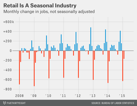
This would compute the difference in sales from every day to the same day in a previous week. Difference functions allow us to identify seasonal changes when we see repeated up or downswings.
The following plot of the month to month change (diff) in jobs from FiveThirtyEight helps identify the seasonal component to a number of retail jobs:
Pandas Expanding Functions
In addition to the set of rolling_* functions, Pandas also provides a similar collection of expanding_* functions, which, instead of using a window of N values, uses all values up until that time.
For example,
pd.expanding_mean(daily_store_sales)
computes the average sales, from the first date until the date specified. Meanwhile:
pd.expanding_sum(daily_store_sales)
computes the sum of average sales per store up until that date.
INSTRUCTOR NOTE: The solution code for these questions can be found below as well in the solution code notebook.
- Plot the distribution of sales by month and compare the effect of promotions.
- Are sales more correlated with the prior date, a similar date last year, or a similar date last month?
- Plot the 15 day rolling mean of customers in the stores.
- Identify the date with largest drop in sales from the same date in the previous month.
- Compute the total sales up until Dec. 2014.
- When were the largest differences between 15-day moving/rolling averages? HINT: Using
rolling_meananddiff
- Plot the distribution of sales by month and compare the effect of promotions
sb.factorplot(
    col='Open',
    hue='Promo',
    x='Month',
    y='Sales',
    data=store1_data,
    kind='box'
)
- Are sales more correlated with the prior date, a similar date last year, or a similar date last month?
# Compare the following:
average_daily_sales = data[['Sales', 'Open']].resample('D', how='mean')

average_daily_sales['Sales'].autocorr(lag=1)

average_daily_sales['Sales'].autocorr(lag=30)

average_daily_sales['Sales'].autocorr(lag=365)
- Plot the 15 day rolling mean of customers in the stores:
pd.rolling_mean(data[['Sales']], window=15, freq='D').plot()
- Identify the date with largest drop in average store sales from the same date in the previous month:
average_daily_sales = data[['Sales', 'Open']].resample('D', how='mean')
average_daily_sales['DiffVsLastWeek'] = average_daily_sales[['Sales']].diff(periods=7)

average_daily_sales.sort(['DiffVsLastWeek']).head
Unsurprisingly, this day is Dec. 25 and Dec. 26 in 2014 and 2015, when the store is closed and there are many sales in the preceding week. How about when the store is open?
average_daily_sales[average_daily_sales.Open == 1].sort(['DiffVsLastWeek'])
The top values are Dec. 24th, but sales on 2013-12-09 and 2013-10-14 were on average 4k lower than the same day in the previous week.
- Compute the total sales up until Dec. 2014:
total_daily_sales = data[['Sales']].resample('D', how='sum')
pd.expanding_sum(total_daily_sales)['2014-12']
Note that this is NOT
pd.expanding_sum(data['Sales'])['2014-12']
because we do not want to sum over our stores first.
- When were the largest differences between 15-day moving/rolling averages?
HINT: Using
rolling_meananddiff
pd.rolling_mean(total_daily_sales, window=15).diff(1).sort('Sales')
Unsurprisingly, they occur at the beginning of every year after the holiday season.
Conclusion (5 mins)
- We use time series analysis to identify changes in values over time
- We want to identify whether changes are true trends or seasonal changes
- Rolling means give us a local statistic of an average in time, smoothing out random fluctuations and removing outliers
- Autocorrelations are a measure of how much a data point is dependent on previous data points